AdversarialCatTF

神经网络如何看待一只猫#

一个在 ImageNet 上预训练的神经网络能够识别多达 1000 种不同类别的物体，比如不同品种的猫。很有趣的是，看看神经网络眼中的理想暹罗猫是什么样子。

当然，你可以将暹罗猫替换为 ImageNet 中的任何其他类别。

首先，让我们加载 VGG 网络：

In [1]:

import tensorflow as tf
from tensorflow import keras
import matplotlib.pyplot as plt
import numpy as np
from IPython.display import clear_output
from PIL import Image
import json
np.set_printoptions(precision=3,suppress=True)

model = keras.applications.VGG16(weights='imagenet',include_top=True)
classes = json.loads(open('imagenet_classes.json','r').read())

2022-06-17 13:28:58.931467: I tensorflow/core/platform/cpu_feature_guard.cc:151] This TensorFlow binary is optimized with oneAPI Deep Neural Network Library (oneDNN) to use the following CPU instructions in performance-critical operations:  AVX2 FMA
To enable them in other operations, rebuild TensorFlow with the appropriate compiler flags.
2022-06-17 13:28:59.603736: I tensorflow/core/common_runtime/gpu/gpu_device.cc:1525] Created device /job:localhost/replica:0/task:0/device:GPU:0 with 15401 MB memory:  -> device: 0, name: Tesla P100-PCIE-16GB, pci bus id: 0001:00:00.0, compute capability: 6.0

优化结果#

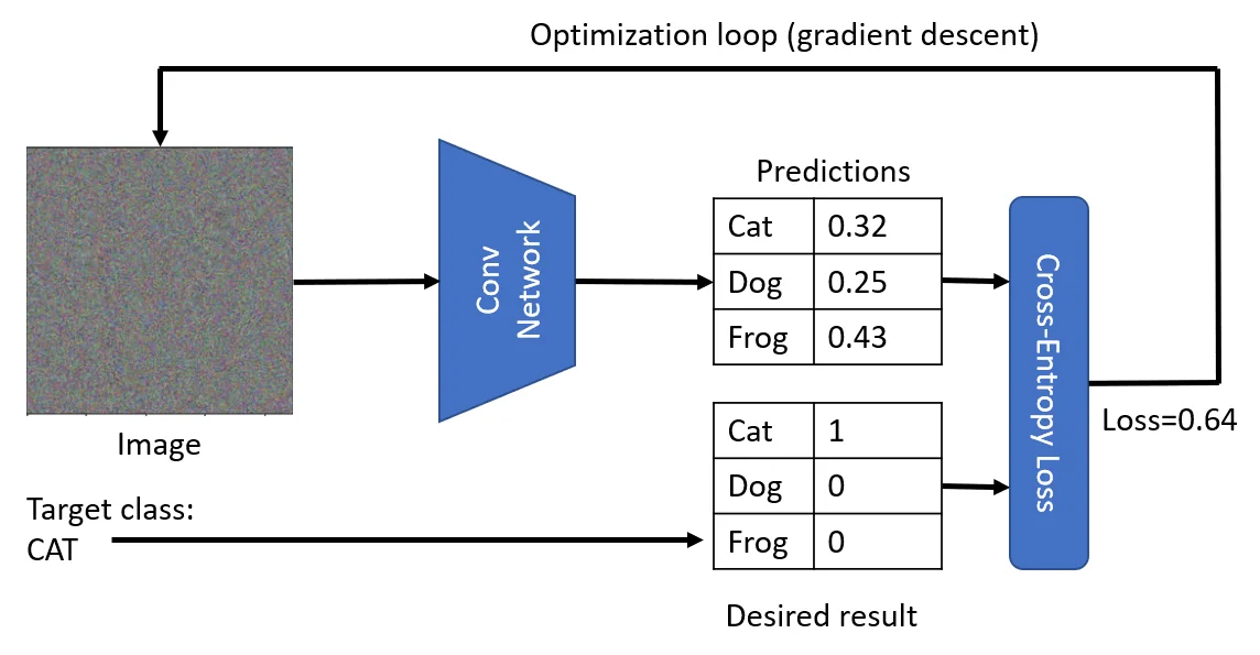
为了呈现理想的猫，我们将从一张随机噪声图像开始，并尝试使用梯度下降优化技术调整图像，使网络能够识别出一只猫。

优化循环

这是我们的起始图像：

In [2]:

x = tf.Variable(tf.random.normal((1,224,224,3)))

def normalize(img):
    return (img-tf.reduce_min(img))/(tf.reduce_max(img)-tf.reduce_min(img))

plt.imshow(normalize(x[0]))

<matplotlib.image.AxesImage at 0x7f90a0277ac0>

我们使用 normalize 函数将我们的值调整到 0-1 范围内。

如果我们在这张图片上调用我们的 VGG 网络，我们将得到一个或多或少随机分布的概率：

In [3]:

def plot_result(x):
    res = model(x)[0]
    cls = tf.argmax(res)
    print(f"Predicted class: {cls} ({classes[cls]})")
    print(f"Probability of predicted class = {res[cls]}")
    fig,ax = plt.subplots(1,2,figsize=(15,2.5),gridspec_kw = { "width_ratios" : [1,5]} )
    ax[0].imshow(normalize(x[0]))
    ax[0].axis('off')
    ax[1].bar(range(1000),res,width=3)
    plt.show()

plot_result(x)

2022-06-17 13:29:02.100818: I tensorflow/stream_executor/cuda/cuda_dnn.cc:368] Loaded cuDNN version 8303
2022-06-17 13:29:02.570980: I tensorflow/core/platform/default/subprocess.cc:304] Start cannot spawn child process: No such file or directory

Predicted class: 669 (mosquito net)
Probability of predicted class = 0.05466596782207489

尽管看起来某个类别的概率比其他类别高得多，但实际上它仍然很低——查看刻度可以发现实际概率仍然在5%左右。

现在我们选择一个目标类别（例如，暹罗猫），并开始使用梯度下降来调整图像。如果 $x$ 是输入图像，$V$ 是 VGG 网络，我们将计算损失函数 $\mathcal{L} = \mathcal{L}(c,V(x))$（其中 $c$ 是目标类别），并使用以下公式调整 $x$： $$ x^{(i+1)} = x^{(i)} - \eta{\partial \mathcal{L}\over\partial x} $$ 损失函数将使用交叉熵损失，因为我们在比较两个概率分布。在我们的例子中，由于类别是用数字表示的，而不是用独热编码向量表示的，我们将使用稀疏分类交叉熵。

我们将重复这个过程若干个周期，并在过程中打印图像。

最好在支持 GPU 的计算设备上运行这段代码，或者减少周期数以缩短等待时间。

In [4]:

target = [284] # Siamese cat

def cross_entropy_loss(target,res):
    return tf.reduce_mean(keras.metrics.sparse_categorical_crossentropy(target,res))

def optimize(x,target,epochs=1000,show_every=None,loss_fn=cross_entropy_loss, eta=1.0):
    if show_every is None:
        show_every = epochs // 10
    for i in range(epochs):
        with tf.GradientTape() as t:
            res = model(x)
            loss = loss_fn(target,res)
            grads = t.gradient(loss,x)
            x.assign_sub(eta*grads)
            if i%show_every == 0:
                clear_output(wait=True)
                print(f"Epoch: {i}, loss: {loss}")
                plt.imshow(normalize(x[0]))
                plt.show()

optimize(x,target)

Epoch: 900, loss: 0.5220473408699036

In [5]:

plot_result(x)

Predicted class: 284 (Siamese cat, Siamese)
Probability of predicted class = 0.6449142098426819

我们现在已经为神经网络获得了一张看起来像猫的图像，尽管对我们来说它仍然像是噪声。如果我们再优化一段时间——很可能会得到一张理想的噪声猫图像，其概率接近1。

理解噪声#

这种噪声对我们来说意义不大，但它很可能包含了许多典型于猫的低级滤波器。然而，由于优化输入以获得理想结果的方法非常多，优化算法并没有动力去寻找那些视觉上易于理解的模式。

为了让图像看起来不那么像噪声，我们可以在损失函数中引入一个额外的项——变化损失。它衡量图像中相邻像素的相似程度。如果我们将这一项加入到我们的损失函数中，它会迫使优化器找到噪声更少的解决方案，从而包含更多可识别的细节。

实际操作中，我们需要在交叉熵损失和变化损失之间找到平衡，以获得良好的结果。在我们的函数中，我们引入了一些数值系数，你可以调整这些系数并观察图像的变化。

In [6]:

def total_loss(target,res):
    return 10*tf.reduce_mean(keras.metrics.sparse_categorical_crossentropy(target,res)) + \
           0.005*tf.image.total_variation(x,res)

optimize(x,target,loss_fn=total_loss)

Epoch: 900, loss: [27.257]

这是我们神经网络理想的猫的图像，我们也可以看到一些熟悉的特征，比如眼睛和耳朵。它们有很多，这使得神经网络更加确信这是一只猫。

In [7]:

plot_result(x)

Predicted class: 284 (Siamese cat, Siamese)
Probability of predicted class = 0.9201651215553284

让我们看看 VGG 对其他一些对象的表现如何：

In [8]:

x = tf.Variable(tf.random.normal((1,224,224,3)))
optimize(x,[340],loss_fn=total_loss) # zebra

Epoch: 900, loss: [29.59]

对抗攻击#

由于理想猫图像可能看起来像随机噪声，这表明我们或许可以稍微调整任何图像，使其类别发生变化。让我们稍微实验一下这个想法。我们将从一张狗的图像开始：

In [9]:

img = Image.open('images/dog-from-unsplash.jpg')
img = img.crop((200,20,600,420)).resize((224,224))
img = np.array(img)
plt.imshow(img)

<matplotlib.image.AxesImage at 0x7f8fd816e0a0>

我们可以看到这张图片显然被识别为一只狗：

In [10]:

plot_result(np.expand_dims(img,axis=0))

Predicted class: 171 (Italian greyhound)
Probability of predicted class = 0.9281901121139526

现在，我们将以此图像为起点，并尝试将其优化成一只猫：

In [11]:

x = tf.Variable(np.expand_dims(img,axis=0).astype(np.float32)/255.0)
optimize(x,target,epochs=100)

Epoch: 90, loss: 0.15769274532794952

In [12]:

plot_result(x)

Predicted class: 284 (Siamese cat, Siamese)
Probability of predicted class = 0.8651191592216492

所以，从 VGG 网络的角度来看，上面的这张图片是一只完美的猫！

使用 ResNet 进行实验#

现在让我们看看这张图片是如何被另一个模型（比如 ResNet）分类的：

In [13]:

model = keras.applications.ResNet50(weights='imagenet',include_top=True)

由于我们将 model 用作全局变量，从现在开始所有函数将使用 ResNet 而不是 VGG

In [14]:

plot_result(x)

Predicted class: 111 (nematode, nematode worm, roundworm)
Probability of predicted class = 0.13089127838611603

显然，结果非常不同。这是可以预料的，因为在针对猫进行优化时，我们考虑了VGG网络的特性、它的低级滤波器等因素。由于ResNet具有不同的滤波器，因此它给出了不同的结果。这让我们产生了一个想法：我们可以通过使用不同模型的集成来保护自己免受对抗性攻击。

让我们看看在ResNet中理想的斑马是什么样子的：

In [15]:

x = tf.Variable(tf.random.normal((1,224,224,3)))
optimize(x,target=[340],epochs=500,loss_fn=total_loss)

Epoch: 450, loss: [46.166]

In [16]:

plot_result(x)

Predicted class: 340 (zebra)
Probability of predicted class = 0.8876020312309265

这幅图截然不同，告诉我们神经网络的架构可能在其识别物体的方式中起着相当重要的作用。

任务: 尝试对 ResNet 进行对抗攻击，并比较结果。

使用不同的优化器#

在我们的例子中，我们一直在使用最简单的优化技术——梯度下降。然而，Keras 框架包含了不同的内置优化器，我们可以用它们来代替梯度下降。这只需要对我们的代码进行很小的改动——我们将用优化器的 apply_gradients 函数替换调整输入图像 x.assign_sub(eta*grads) 的部分：

In [17]:

def optimize(x,target,epochs=1000,show_every=None,loss_fn=cross_entropy_loss,optimizer=keras.optimizers.SGD(learning_rate=1)):
    if show_every is None:
        show_every = epochs // 10
    for i in range(epochs):
        with tf.GradientTape() as t:
            res = model(x)
            loss = loss_fn(target,res)
            grads = t.gradient(loss,x)
            optimizer.apply_gradients([(grads,x)])
            if i%show_every == 0:
                clear_output(wait=True)
                print(f"Epoch: {i}, loss: {loss}")
                plt.imshow(normalize(x[0]))
                plt.show()

x = tf.Variable(tf.random.normal((1,224,224,3)))

optimize(x,[898],loss_fn=total_loss) # water bottle

Epoch: 900, loss: [41.451]

结论#

我们通过使用梯度下降优化调整输入图像（而非权重），成功在预训练的CNN中可视化了理想的猫的图像（以及其他任何对象）。获得有意义图像的主要技巧是使用变化损失作为附加损失函数，这使得图像看起来更加平滑。

免责声明：
本文档使用AI翻译服务 Co-op Translator 进行翻译。尽管我们努力确保翻译的准确性，但请注意，自动翻译可能包含错误或不准确之处。原始语言的文档应被视为权威来源。对于关键信息，建议使用专业人工翻译。我们不对因使用此翻译而产生的任何误解或误读承担责任。